
The Kalman Filter an Introduction to Concepts
Nearly tutorials for the Kalman Filter are difficult to understand because they require avant-garde math skills to empathise how the Kalman Filter is derived. If you have tried to read Rudolf E Kalman's 1960 Kalman Filter paper, you know how disruptive this concept can exist. But do you demand to empathize how to derive the Kalman Filter in society to use it?
No. If you want to design and implement a Kalman Filter, y'all do not need to know how to derive it, you but demand to sympathise how it works.
The truth is, anybody tin understand the Kalman Filter if information technology is explained in small digestible chunks. This post simply explains the Kalman Filter and how it works to judge the state of a system.
The large picture of the Kalman Filter
Lets look at the Kalman Filter as a black box. The Kalman Filter has inputs and outputs. The inputs are noisy and sometimes inaccurate measurements. The outputs are less noisy and sometimes more than authentic estimates. The estimates tin can exist system state parameters that were not measured or observed. This last sentence describes the super power of the Kalman Filter. Once again, the Kalman Filter estimates system parameters that are not observed or measured.
In brusk, you can retrieve of the Kalman Filter as an algorithm that can estimate observable and unobservable parameters with peachy accurateness in existent-time. Estimates with high accuracy are used to make precise predictions and decisions. For these reasons, Kalman Filters are used in robotics and real-fourth dimension systems that need reliable information.
What is the Kalman Filter?
But put, the Kalman Filter is a generic algorithm that is used to estimate system parameters. Information technology tin can employ inaccurate or noisy measurements to estimate the land of that variable or another unobservable variable with greater accurateness. For instance, Kalman Filtering is used to practise the following:
- Object Tracking – Use the measured position of an object to more accurately estimate the position and velocity of that object.
- Torso Weight Guess on Digital Scale – Apply the measured pressure on a surface to estimate the weight of object on that surface.
- Guidance, Navigation, and Control – Apply Inertial Measurement Unit (IMU) sensors to estimate an objects location, velocity, and acceleration; and use those estimates to control the objects adjacent moves.
The existent power of the Kalman Filter is not smoothing measurements. It is the ability to estimate organisation parameters that can not exist measured or observed with accuracy. Estimates with improved accuracy in systems that operate in real time, allow systems greater control and thus more than capabilities.
Kalman Filter Algorithm Overview
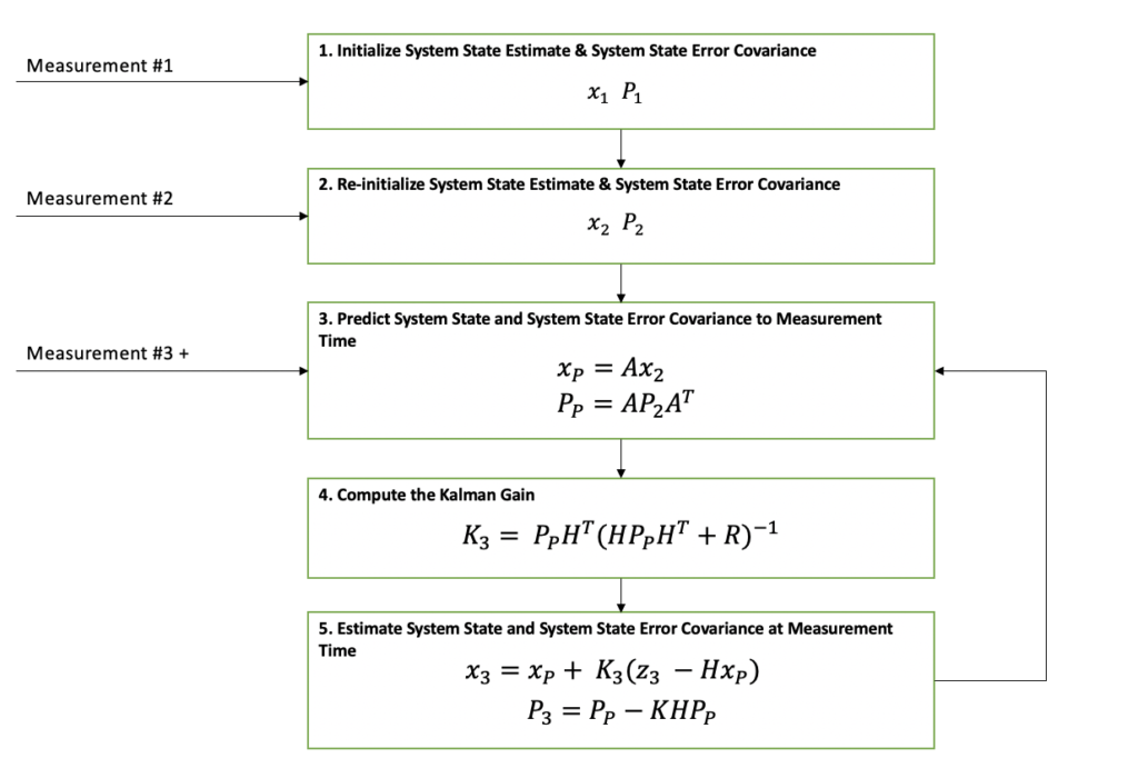
The process diagram to a higher place shows the Kalman Filter algorithm step past footstep. I know those equations are intimidating but I clinch you lot this will all make sense by the time you stop reading this commodity. Allow'due south look at this process ane step at a time. For your reference, hither is a table of definitions that will exist referred to throughout.
| x | state variable | n x i cavalcade vector | Output |
| P | state covariance matrix | northward x n matrix | Output |
| z | measurement | m x 1 cavalcade vector | Input |
| A | state transition matrix | n x due north matrix | Organisation Model |
| H | state-to-measurement matrix | m x due north matrix | Arrangement Model |
| R | measurement covariance matrix | grand ten m matrix | Input |
| Q | process noise covariance matrix | due north x north matrix | System Model |
| G | Kalman Gain | n x m | Internal |
The table above identifies the variables used in the algorithm. Each variable listed has a structure blazon and category. As this article continues, use the table equally a reference.
If you are enjoying this post, bank check out my eBook Kalman Filter Explained Just. Y'all volition learn: the beginning principles behind the Kalman Filter, how to create simulations and perform analysis on Kalman Filters, and more. Or Purchase Me a Java with the link in the bottom right corner so I can keep writing web log posts!
Kalman Filter Radar Tracking Tutorial
This tutorial will go through the footstep past step procedure of a Kalman Filter being used to rail airplanes and objects almost airports. The output track states are used to brandish to the air traffic command operators monitoring the air infinite.
Kalman Filter Tutorial Notation
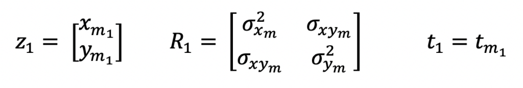
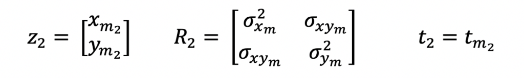
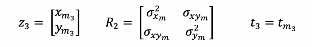
Radars are not congenital equally. Each i has dissimilar capabilities and therefore provides unlike types of information to its supporting systems. For this example, the radar will output its measurements in second cartesian coordinates, 10 and y. These measurements will be represented every bit a 2-by-1 column vector, z. The associated variance-covariance matrix for these measurements, R, will also be provided past the radar forth with the time tag for when the measurement occurred, t. The subscript m denotes the measurement parameters. And the one thousand subscript denotes the gild of the measurement.
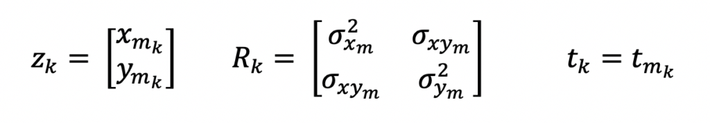
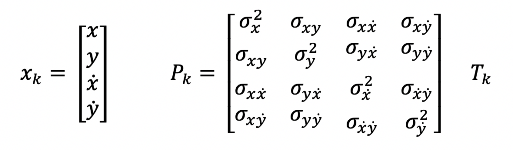
The Kalman Filter estimates the objects position and velocity based on the radar measurements. The estimate is represented by a 4-by-1 cavalcade vector, x. It's associated variance-covariance matrix for the gauge is represented past a four-past-4 matrix, P. Additionally, the state estimate has a time tag denoted equally T.
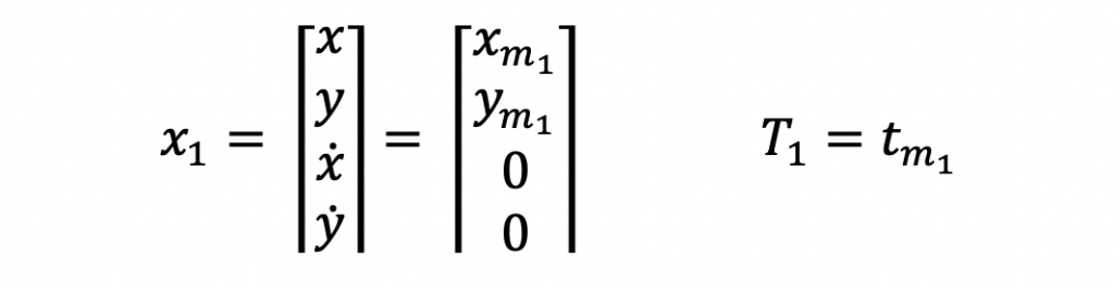
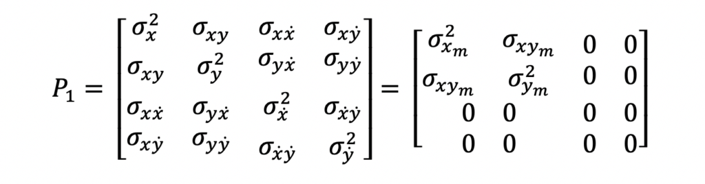
Stride 1: Initialize Arrangement State
Initializing the arrangement state of a Kalman Filter varies across applications. In this tutorial, the Kalman Filter initializes the system state with the first measurement.
| xchiliad | Eqn. i-1 |
| Pk | Eqn. i-ii |
In this radar tracking instance, the input measurements contain position only information. The output system state volition incorporate the position and velocity of the object.
When the first measurement comes, the only information known about the object is the position at that point in fourth dimension. The system state estimate volition be fix to the input position after the first judge. The system country error covariance will be set to the beginning measurement's position accuracy.
Initialize System State in Equations
These equations show the input and output values for this Kalman Filter later receiving the outset measurement.
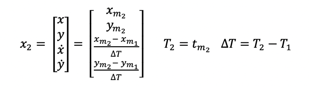
Footstep 2: Reinitialize System Country
The system state estimate is reinitialized considering a velocity estimate needs a second position measurement for computation.
| xone thousand | Eqn. ii-1 |
| Pk | Eqn. 2-2 |
Velocity is estimated with a linear approximation. Equally you most likely recall from high school physics, velocity is equal to the altitude traveled divided by the time information technology took to travel that distance.
The updated system land estimate will be the second measurement'southward position and the computed velocity. The updated organization country error covariance will be the second measurement'southward position accurateness and an approximated velocity accuracy. Annotation that this velocity accuracy approximation is something that tin can exist tuned and adjusted after running data through your filter. There are dissimilar ways of approximating these values so if this doesn't match your approximation, that'south okay!
Reinitialize Arrangement Country in Equations
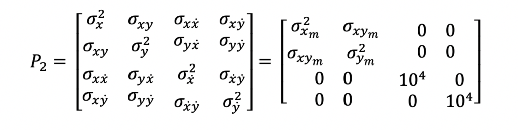
These equations show the input and output values for this Kalman Filter after receiving the 2d measurement. Annotation the velocity variance terms in the state covariance matrix. These values are being set to ten4. In other words, this value indicates a large uncertainty for the velocity country values. In this case, the velocity units are meters per second.
Quick Note on Initialization
Steps one and 2 used the outset couple measurements to initialize and re-initialize the system judge. Each application of the Kalman Filter may practice this differently but the goal is to have a system state estimate that can exist updated for futurity measurement with the Kalman Filter equations.
Steps 3 through 6 demonstrate how measurements are filtered in and the country estimate is updated.
Step iii: Predict System State Estimate
When the third measurement is received, the system state estimate is propagated forwards to time align it with the measurement. This alignment is done so that the measurement and state estimate tin can exist combined.
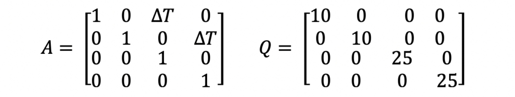
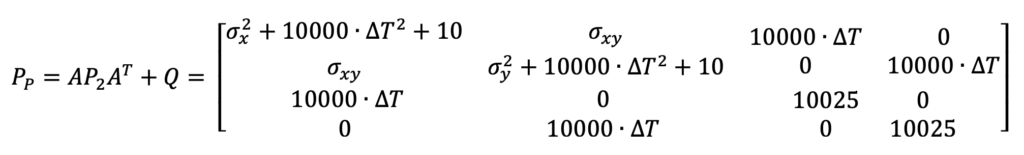
| 10p = Axg-1 | Eqn. iii-1 |
| Pp = APg-aneAT + Q | Eqn. 3-ii |
The organisation model is used to perform this prediction. In this instance, a constant velocity linear motion model is used to approximate the objects position change over a time interval. Notation that a abiding velocity model does presume zero acceleration. Remember this because it will resurface later.
The constant velocity linear motion model is something you may also remember from your high school physics class. The equation states that the position of an object is equal to its initial position plus its displacement over a specified fourth dimension period assuming a constant velocity.
A country transition matrix represents these equations. This matrix is used to propagate the land estimate and state error covariance matrix appropriately. You may be wondering why the state mistake covariance matrix is propagated. The reason for this is because when a state approximate is propagated in time, the dubiousness about its land at this future time stride is inherently uncertain, so the error covariance grows.
On the Q Matrix
The Q matrix represents process racket for the system model. The organization model is an approximation. Throughout the life of a system land, that system model fluctuates in its accurateness. Therefore, the Q matrix is used to stand for this uncertainty and adds to the existing dissonance on the country. For this example, the systems actual accelerations and decelerations contribute to this fault.
On the H Matrix
The Kalman Filter uses the land-to-measurement matrix, H, to convert the system state estimate from the state space to the measurement space. For some Kalman Filter applications, this is a matrix of zeros and ones. For other applications that use the Extended Kalman Filter, the H matrix is populated with differential equations. To learn more nearly Extended Kalman Filters, check out my article on them here.
In this tutorial, the H matrix is a simple matrix that is set up up to reduce the state approximate and fault covariance to position only values rather than position and velocity.
Predict System Land in Equations


Step 4: Compute the Kalman Proceeds
The Kalman Filter computes a Kalman Gain for each new measurement that determines how much the input measurement will influence the organisation state estimate. In other words, when a actually noisy measurement comes in to update the system country, the Kalman Gain will trust its current state gauge more than than this new inaccurate information.
This concept is the root of the Kalman Filter algorithm and why it works. It tin recognize how to properly weight its electric current approximate and the new measurement information to form an optimal estimate.
| K = PPHT (HPPHT + R )-1 | Eqn. four-i |
Step 5: Gauge Arrangement State and System State Error Covariance Matrix
The Kalman Filter uses the Kalman Gain to estimate the system state and fault covariance matrix for the time of the input measurement. After the Kalman Gain is computed, it is used to weight the measurement appropriately in 2 computations.
The outset computation is the new organization state guess. The second computation is the organisation state error covariance.
| xk = xp + M(zk – Hxp) | Eqn. 5-i |
| Pk = PP – KHPP | Eqn. five-two |
The country approximate computed above is the only country history the Kalman Filter retains. Every bit a effect, Kalman Filters can exist implemented on machines with low memory restrictions.
If y'all enjoyed reading this post, cheque out my eBook Kalman Filter Made Like shooting fish in a barrel. You will learn: the first principles behind the Kalman Filter, how to create simulations and perform assay on Kalman Filters, and more.
Side by side Steps
I hope this post allowed yous to come across how amazing the Kalman Filter is. And when it is broken up into parts, information technology is not that intimidating.
In decision, the Kalman Filter is a generic procedure for optimal state estimation. It is used in a variety of applications that crave authentic estimation. Then now that you know what information technology is and how it works, go out and use it in your projects!
If you enjoyed reading this post, please share it with your friends on your favorite social network! Thanks for reading!
The Kalman Filter an Introduction to Concepts
Posted by: bealeforris.blogspot.com